8  Faceting

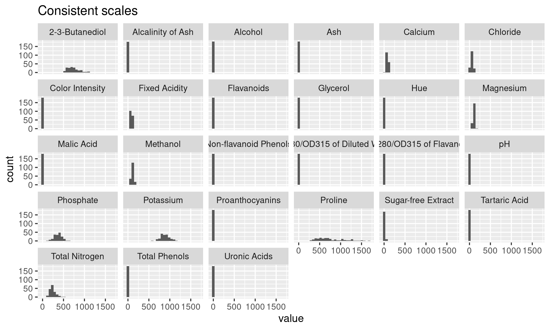
In this chapter, we will introduce faceting, a technique that produces multiple plots in which the data is subsetted by a categorical feature.

8.1 Faceting on one variable: facet_wrap()

ggplot(iris, aes(Sepal.Length, Sepal.Width)) +  
  geom_point(color = "cornflowerblue") +  
  facet_wrap(~Species)

To control the layout dimensions, you can choose the number of rows or columns (nrow = or ncol =).

8.2 Reordering facets

Facets are ordered according to the factor level order of the faceted variable. See the chapter on factors for strategies on reordering factor levels.

library(MASS)
painters |> 
  rownames_to_column("Name") |> 
  filter(School == "A") |> 
  pivot_longer(Composition:Expression, names_to = "Skill",
               values_to = "Score") |> 
  ggplot(aes(x = Score, y = fct_reorder(Name, Score))) +
  geom_point(color= "#786FB8") +
  facet_wrap(~Skill, ncol = 1)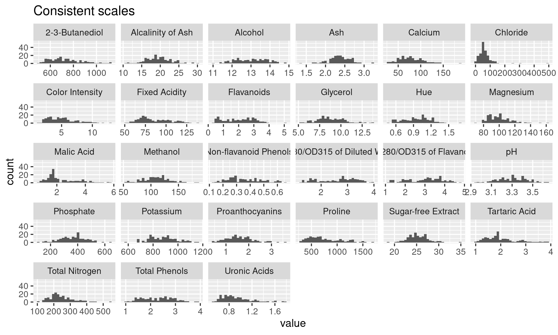

birds_plot <- birds |> 
  group_by(phase_of_flt) |> 
  summarize(count = n()) |> 
  slice_max(order_by = count, n = 4)

Error: object 'birds' not found

ggplot(birds, aes(x = speed, y = after_stat(density))) + 
  geom_histogram() +
  facet_wrap(~phase_of_flt, nrow = 1)

Error: object 'birds' not found

8.3 Faceting on two variables: facet_grid()

With two variables, the rows represent the levels of one variable and the columns the other. These can be specified with the formula notation: facet_wrap(row variable~column variable).

library(scales)
library(openintro)

Error in library(openintro): there is no package called 'openintro'

ggplot(cle_sac, aes(x = age, y = personal_income)) +
  geom_point(size = 1, color = "cornflowerblue") +
  facet_grid(sex ~ city) +
  scale_y_continuous(labels = unit_format(unit = "K", scale = .001)) +
  labs(x = "age (in years)", y = "personal income", 
       caption = "Data: openintro::cle_sac") +
  theme_bw(16)

Error: object 'cle_sac' not found

8.4 Faceting with categorical variables

library(pgmm) 
data(wine)  
tidywine <- wine |> 
  pivot_longer(cols = -Type, names_to = "variable",
               values_to = "value")  
tidywine |>
  ggplot(aes(value)) +
  geom_histogram(color = "blue", fill = "cornflowerblue",
                 bins = 20) +
  facet_wrap(~variable) +
  labs(title = "Fixed scales (default)") +
  theme_grey(14)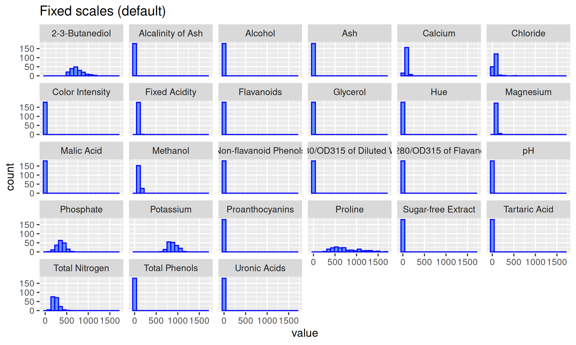

Axis scales can be made independent, by setting scales to free, free_x, or free_y.

In this case, scales = "free_x" is a better option because the distribution of each numerical variable is more obvious.

tidywine |>
  ggplot(aes(value)) +
  geom_histogram(color = "blue", fill = "cornflowerblue",
                 bins = 20) +
  facet_wrap(~variable, scales = "free_x") +
  labs(title = "Free x scale") +
  theme_grey(14)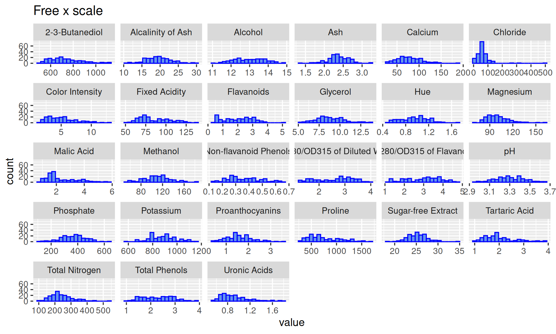

8.5 Faceting on two variables

facet_grid can be used to split data-sets on two variables and plot them on the horizontal and/or vertical direction.

wine |>   
  mutate(Type = paste("Type", Type)) |>   
  select(1:6) |>   
  pivot_longer(cols = -Type, names_to = "variable", values_to = "value") |>  
  ggplot(aes(value)) +  
  geom_histogram(color = mycol, fill = "lightblue") +  
  facet_grid(Type ~ variable, scales = "free_x") +  
  theme_grey(14)

Error in select(mutate(wine, Type = paste("Type", Type)), 1:6): unused argument (1:6)